Zachariah W Miller, PhD

Physics Analysis Tree Maker

November 27, 2016 - C++

One of the great challenges of working with large-scale detectors like the STAR detector is the sheer volume of data that one must organize and control. One of my main contributions to the analyses of our group at University of Illinois at Chicago is the implementation and maintenance of a code project that helps manage all of that data. To help understand that project, I think it's worthwhile to understand the full "path" of the data as we go from particle collisions to results. The image below will help show how that works. 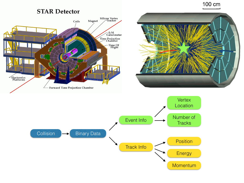At the top-left is a schematic of the STAR detector. There are many detector systems, but I'd like to highlight the Time Projection Chamber (TPC) and the Barrel Electron-Magnetic Calorimeter (BEMC; listed as E-M Calorimeter). For the purposes of this discussion, I will be focusing on these detectors. The TPC is a large chamber filled with a gas that ionizes when a charged particle moves through it. This chamber has both an electric and magnetic field applied throughout. This force the ionized gas to "float" toward the ends of the detector where it can be collected and converted into digital information that tells us where the particle was and how it was moving. The E-M Calorimeter is a large barrel of plastic detectors. When a particle is stopped by interacting with the plastic, it releases light. This light can be collected and converted into digital data that tells us the energy of the particle. All of the data from these detectors, are what we will focus on keeping in our analyses.

In the top-right is a diagram of a typical particle collision event. I've added a star to show where the collision occurred in this event. All of the yellow lines are individual particles coming out of the collision. These are called "tracks" and the collision is known as the "vertex." When an event occurs, each of these tracks is actually just a chain of ionization within the gas, and perhaps an interaction within the BEMC. For our analyses we want to have a set of tracks associated with an event, and each track and event should have well-known physical properties that we extract from the data, as shown in the simplified flow chart.

This is where the large amount of data comes from. There can be hundreds of tracks and each one has dozens of hits in the TPC from ionized gas collection. Each hit is categorized by at least four 11-bit values. Beyond that, there are thousands of BEMC panels, and each one of these must be read out and some determination of whether that panel belongs to a track must be done (each of these read-outs will be dozens of 11-bit values). That's just two of the many detectors that make up STAR. From there, STAR has a conversion from binary "readout" data to the tracks and event objects, with many values associated with each. Some of these are the converted raw data, but we also calculate many more variables to fully characterize each object. We do this over and over for millions upon millions of events. When all is said and done, for a given dataset we may have 100s of terabytes worth of information saved. This all happens as part of event reconstruction before analyzers ever see the data and can make decisions about what to keep. So, just in the baseline, we already have a huge dataset.

And there-in lies a new challenge. Physics analyses are quite iterative, we might process all the data once to see what changes we need to make to select different particles or how to select events better or... and then repeat these iterations for months. Iterating over 100s of terabytes can take an extreme amount of time that is prohibitive to analysis. With this in mind, Bingchu Huang and I designed a method to minimize the amount of data we actually need to iterate over. This method takes advantage of the tree structure in ROOT which is a form of Tuple. The two main ideas for this code is to only keep the information necessary for our analysis instead of keeping all of the data for each track and to minimize the memory usage of each data structure by limiting the precision when possible.

Necessary Information

The first key is to minimize the number of "junk" events in our dataset. There are a few bits of information that we want to consider when considering whether to keep an event or not. The first is whether the vertex position (where the collision occurs) is in a region that is close enough to the center of the detector that the detector works at optimal efficiency. This is the "Vz" distribution shown at left. We want to select a region around 0 cm, with some reasonable, but fairly non-restrictive width, such that each analysis can set a tighter cut if necessary. For this example, a cut around 40 cm would keep the vast majority of the data and still be loose enough for future optimization. It will still help remove some of the "junk" events that are far from the center.

Besides the TPC, there is another detector called the "Vertex Position Detector (VPD)" that also tracks where the collision occurs. Thus, another key method for removing bad events is to check if both vertex finding detectors agree on the position of the vertex. The plot at right shows the correlation between the two detectors on the Z-position of the vertex. We can make a cut perpendicular to the correlation by selecting only events where there is a 1:1 correlation, within some tolerance. These requirements help us to remove useless events that are technically "true" events, but that will not be useful in our analysis.

In STAR's main data format, every possible piece of information for each track is recorded. This is a massive waste of space if you are only interested in certain tracks or certain pieces of information about the tracks. In order to reduce this, our code splits tracks into multiple sub-classes, and each class only records the information necessary. As an example, in my analysis we are most interested in electrons so for electrons we want to record many pieces of data. So we make a loose, "on-the-fly" check if a track is an electron candidate and if so, we store it as an electron class object. In this class, we keep all the information to identify electrons, the position of the electron's starting point relative to the vertex, all of the kinematic information, etc. However, for other tracks where we are only going to compare kinematic information to establish correlations, we have no need to keep the particle indentification information. We can do a similar method for identifying muons, pions, and kaons; creating a class for each of the track types and deciding what data each type requires. How we identify these particles is worth a separate discussion, but a quick example can be seen at left. This shows the energy loss of all tracks in the TPC. You can see there are many different bands, and each band corresponds to a different type of particle for a given momentum (P). By making selections on variables like this (and others like time between collision and interaction with BEMC), we can make loose selections on particle type and only save the necessary information for a given track type.

Another key is to only keep tracks that are physically useable. The key to this is a physical understanding of the detector. Given the large magnetic field, a charged particle will be forced to move in a circle inside the cylindrical detector. If the particle does not have enough energy to make a circle with a radius large enough to reach the outside of the detector, it will spiral until it leaves the detector and not be a collected correctly. To overcome this, we can require that the tracks we analyze have some minimum momentum. This is a huge memory savings due to the distribution of track momenta, as shown at right. The vast majority of tracks have small momentum, so if we do an initial screening to remove those tracks that have a momentum below the usable range for our analyses, we can remove lots of tracks that we'd later have to remove during each iteration.

Minimizing Precision

The other method we use for memory management is to mimimize the precision of the stored value. The natural way to store the information is to just assign each value for each track as a C++ float. However, this may not be necessary for some values. As an example, when looking at the distance between the vertex and a track's starting point, we know that the detector has a resolution of a few millimeters. Thus, if we save a float that extends out into nanometer acccuracy, it's actually just storing meaningless values in many of the digits. In order to minimize this "junk," we can store the values as an integer or a short by multiplying the float value by some "encoding" value and providing a decoding function to access the value. This is shown below as an example:


This example shows a method of encoding a float to a short, lowering the memory requirement by 1/2 while not losing any "real" information due to the detectors resolution being at the 1/1000th scale. This can be done for almost every piece of information for every track. For an analyzer, this just means that they cannot directly load a class object and access the member variables, but must instead access the values through a "getter" function (which is actually a bit safer such that no value is ever accidentally over-written).

Summary

So, how well does this work? Luckily, it's an easy result to quantify, since we have access to the before and after size of the data. The STAR official production for the Run 15 p+p collision data has a size of over 300 TB. After conversion to the ROOT "analysis tree" that our analyses are based upon, we only store about 5 TB of data. A reduction by a factor of ~60. Similar results are seen for other datasets as well. Even more importantly, when we iterate through the data on the computing cluster the analysis tree takes less than 6 hours, while the full data takes almost a week!

Admittedly, the functionality of this code is limited. It is only designed to only prepare an analysis tree for our specific needs, as we've customized this output to be prepared for our work. However, we now have 6 analyses based on these trees, meaning that the result of this code is being used to look at dozens of physics puzzles at the moment. The ability to collate and prune the mass of data from STAR into small, usable clusters is key to making our group competitive in the physics analysis world; and the analysis tree maker has been very successful in providing us this ability. The code could be adapted by others to suit there needs quite simply by just changing what variables are stored in each particle class type (e.g. for pions, I'd like to keep X instead of Y or Z), but we have not yet attempted to globalize the effort.

Code available here.